How to Rank GA4 Channels with PCA, Determinants and Eigenvectors
What eigenvalues, determinants and a 1980s decision-making method can tell you about your traffic channels that a pivot table can’t.
Here’s a table you’ve probably looked at a hundred times. It’s a standard GA4 traffic acquisition export, the starting point for most GA4 channel analysis: ten default channel groups, six metrics.
| Channel | Sessions | Engaged sessions | Engagement rate | Avg engagement time (s) | Conversions | Key event rate |
|---|---|---|---|---|---|---|
| Direct | 18,601 | 13,901 | 74.73% | 34 | 132 | 0.60% |
| Organic Search | 6,971 | 3,462 | 49.66% | 55 | 106 | 1.20% |
| Referral | 670 | 357 | 53.28% | 114 | 10 | 1.19% |
| Organic Social | 522 | 192 | 36.78% | 24 | 19 | 2.11% |
| Unassigned | 330 | 116 | 35.15% | 160 | 2 | 0.30% |
| 187 | 65 | 34.76% | 59 | 49 | 12.83% | |
| AI Assistant | 165 | 70 | 42.42% | 31 | 0 | 0.00% |
| Organic Shopping | 95 | 71 | 74.74% | 159 | 8 | 6.32% |
| Organic Video | 78 | 59 | 75.64% | 54 | 2 | 1.28% |
| Display | 13 | 5 | 38.46% | 66 | 0 | 0.00% |
The usual way to read this: sort by Sessions, say “Direct and Organic are carrying us,” glance at Email’s conversion rate, nod, close the tab.
But you’re comfortable with math, so let’s try something different. That table is a 10 × 6 matrix. Think of it as a spreadsheet where every number has a fixed address (row = channel, column = metric), which lets you run operations on the whole thing at once instead of eyeballing cells one by one.
Once you see it that way, linear algebra gives you three questions you can ask that a dashboard won’t answer:
- What’s actually going on here, in fewer dimensions? (PCA, using eigenvalues and eigenvectors)
- Am I tracking the same thing six times? (correlation matrix and its determinant)
- If I had to rank these channels on everything at once, what would the ranking be? (eigenvector-based ranking, AHP-style)
Let’s go one at a time.
Part 1: Squashing six metrics into two (PCA)
The problem you already have
Six metrics is too many to hold in your head. Honestly, nobody “compares channels across six KPIs.” What you actually do is pick one or two you care about and ignore the rest. PCA does the same thing, but it picks based on where the information actually is, not on gut feel.
Step 1: Put everyone on the same scale
Sessions range from 13 to 18,601, while key event rate ranges from 0 to 12.83. If you don’t fix that, Sessions will steamroll everything else purely because its numbers are bigger.
So we standardize, turning each value into a standard score. Think of it as grading every metric on a curve: each channel’s score becomes “how many standard deviations above or below average.” After that, a +2 on Sessions and a +2 on Engagement rate mean the same thing: unusually high.
The code uses pandas to load the CSV (with read_csv) and NumPy for the math.
import numpy as np
import pandas as pd

df = pd.read_csv('traffic-data.csv')
for col in ['Engagement rate', 'Session key event rate']:
    df[col] = df[col].str.rstrip('%').astype(float)

X = df.iloc[:, 1:].values.astype(float)       # 10 x 6 matrix
Z = (X - X.mean(axis=0)) / X.std(axis=0)      # standardize each column
Step 2: Find the directions that matter
Next we build the covariance matrix (with np.cov), a 6 × 6 grid where each cell tells you whether two metrics tend to rise and fall together. Then we pull out its eigenvectors and eigenvalues with np.linalg.eigh, NumPy’s eigen-solver for symmetric matrices.
Here’s the friend-at-a-bar version. Imagine your data as a cloud of points floating in six-dimensional space. An eigenvector is a direction you could point a flashlight through that cloud, and its eigenvalue tells you how stretched out the cloud is along that direction. The biggest eigenvalue marks the direction where your channels differ the most, which is the direction carrying the most information.
cov = np.cov(Z, rowvar=False)
eigenvalues, eigenvectors = np.linalg.eigh(cov)

order = np.argsort(eigenvalues)[::-1]          # biggest first
eigenvalues, eigenvectors = eigenvalues[order], eigenvectors[:, order]
Each new direction is called a principal component (PC). Here’s how much of the total spread each one captures:
| Component | Eigenvalue | % of variance | Cumulative |
|---|---|---|---|
| PC1 | 3.57 | 53.5% | 53.5% |
| PC2 | 1.24 | 18.6% | 72.1% |
| PC3 | 1.14 | 17.1% | 89.2% |
| PC4 | 0.61 | 9.2% | 98.4% |
| PC5 | 0.11 | 1.6% | 100% |
| PC6 | 0.0001 | 0.0% | 100% |
The scree plot
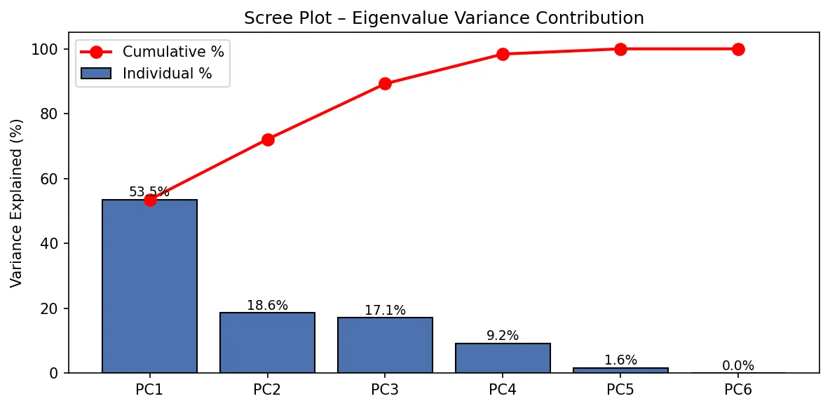
What you’re looking at: each bar is one component’s share of the information, and the red line is the running total.
Why you should care: two numbers per channel get you 72% of the story, and three get you 89%. You’re tracking six metrics, but your channels really only differ in about three meaningful ways. Everything else is mostly echo.
The mental shortcut: whenever someone hands you a dashboard with 15 KPIs, ask, “How many of these are actually independent?” A scree plot answers that. If the curve flattens after bar 3, you need three KPIs, not fifteen.
And look at PC6: an eigenvalue of 0.0001. That’s basically zero, meaning there’s a direction where your data has no spread at all, and no spread means one metric is perfectly predictable from the others. Hold that thought; it comes back in Part 2.
What do the components mean?
An eigenvector is a recipe: it says how much of each original metric goes into a component.
| Metric | PC1 | PC2 |
|---|---|---|
| Sessions | 0.55 | 0.03 |
| Engaged sessions | 0.54 | 0.06 |
| Engagement rate | 0.28 | 0.67 |
| Avg engagement time | −0.24 | 0.70 |
| Conversions | 0.50 | −0.16 |
| Key event rate | −0.12 | −0.14 |
You can just read the labels off this:
- PC1 = “How big is this channel?” Sessions, engaged sessions and conversions all load heavily. It’s a volume score.
- PC2 = “How much do people stick around?” Engagement rate and time on site dominate. It’s an attention score.
(PC3, which isn’t plotted, is almost entirely key event rate at 0.94. That’s your “does this traffic do the thing?” axis. Note that it’s separate from both volume and attention, which is worth remembering.)
The biplot
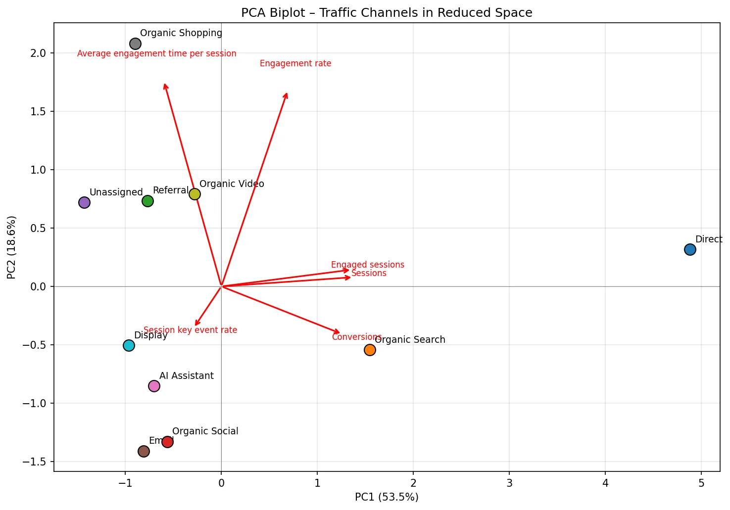
How to read it: in a biplot, every dot is a channel placed by its volume score (x-axis) and attention score (y-axis). The red arrows show which way each original metric “pulls.” Channels that sit close together behave alike across all six metrics.
What jumps out:
- Direct is off in its own postcode at PC1 ≈ 4.9. It’s a different kind of animal from everything else, purely on scale. Comparing it to Display on raw numbers was never a fair fight.
- Organic Search is the only other channel with real positive volume, and it leans toward the Conversions arrow.
- Organic Shopping, Organic Video, Referral and Unassigned cluster up top: small but sticky. People who arrive through them hang around.
- Email, Organic Social and AI Assistant sit in the bottom-left: low volume and low dwell time. But hold on, because Email has the best key event rate in the whole table (12.83%). It just isn’t visible on these two axes, because that signal lives in PC3.
Why you should care: that last point is the lesson. A 2D view can make your best converter look like your worst performer if conversion efficiency lives on an axis you didn’t plot. When you collapse dimensions, always check what fell off.
The mental shortcut for marketing: the biplot is how you find channel personas. Channels that cluster together probably want the same content strategy, the same landing pages and the same success metric. The “small but sticky” cluster (Shopping, Video, Referral) should be judged on depth, not reach. Stop holding them to a sessions target they’ll never hit.
Part 2: Are you tracking the same thing six times?
Correlation, quickly
Correlation (r, Pearson’s correlation coefficient) is a number from −1 to +1 for how tightly two metrics move together. At +1 they’re twins, at 0 they’re strangers, and at −1 they’re on a seesaw.
Put all the pairwise correlations in a 6 × 6 grid and you get the correlation matrix:
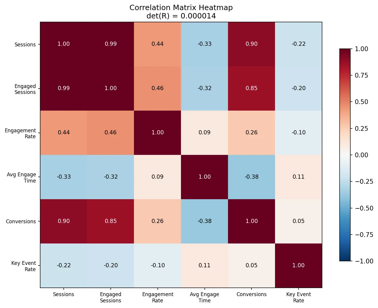
What you’re looking at: dark red means a strong positive relationship, dark blue means negative, and white means unrelated. The diagonal is always 1, since every metric correlates perfectly with itself.
The headline pairs:
| Pair | r | What it means |
|---|---|---|
| Sessions ↔ Engaged sessions | +0.99 | Basically the same number |
| Sessions ↔ Conversions | +0.90 | Conversions mostly track volume |
| Engaged sessions ↔ Conversions | +0.85 | Same story |
| Avg time ↔ Conversions | −0.38 | Longer visits ≠ more conversions |
| Conversions ↔ Key event rate | +0.05 | Totally independent |
That last row is the sneaky one. Conversions (a count) and key event rate (an efficiency) have almost nothing to do with each other. Direct has the most conversions and one of the worst rates, while Email has a tiny count and the best rate by a mile. If your team reports “conversions” and treats that as a quality metric, it’s actually a volume metric in disguise.
The determinant: one number for “how much overlap?”
The determinant squashes a whole square matrix into a single number. For a correlation matrix, it runs from 1 (every metric brings fresh information) down to 0 (at least one metric is a pure rehash of the others). Think of it as a measure of how much elbow room your metrics give each other.
For two metrics it’s easy to see:
| 1.00  0.99 |
| 0.99  1.00 |   det = 1 − 0.99² ≈ 0.02   → nearly the same thing

| 1.00  0.05 |
| 0.05  1.00 |   det = 1 − 0.05² ≈ 0.997  → genuinely different
For our full 6 × 6 matrix:
R = np.corrcoef(X, rowvar=False)
np.linalg.det(R)       # 0.000014
det(R) = 0.000014. That’s about as close to zero as real-world data gets.
A related check is the condition number (largest eigenvalue ÷ smallest). Above 30 is considered trouble, and ours is 44,143.
So what’s the duplicate?
It’s not a mystery. Check the raw data:
Direct: 18,601 sessions × 74.73% engagement rate = 13,900 engaged sessions.
Engaged sessions isn’t a separate measurement. It’s literally Sessions × Engagement rate. (See how GA4 defines engaged sessions and engagement rate.) GA4 hands you all three as if they were independent columns, but one of them is pure arithmetic on the other two. That’s exactly the zero-variance direction PC6 found in Part 1. The math sniffed out a formula hiding in your export without being told about it.
Why you should care
This one has real teeth for marketing teams:
- Scorecards double-count. If your channel scorecard gives equal weight to Sessions, Engaged sessions and Conversions, you’ve given volume three votes and quality one. Big channels win by default.
- Regression and attribution models break. Feed highly correlated inputs into a marketing mix model or a lead-scoring regression (Bayesian ones like the models in the PyMC guide for marketing analysts included) and the coefficients go haywire. They flip signs, balloon, and change wildly when you add a week of data. This is called multicollinearity, and a tiny determinant is the early warning.
- Dashboard bloat. Every redundant KPI costs attention in every meeting.
The mental shortcut: before you build any model or scorecard from a set of metrics, compute np.linalg.det(np.corrcoef(...)) (det, corrcoef). If it’s below about 0.01, you have duplicates. Find them and keep one from each family. In this dataset, a lean, non-redundant set would be: Sessions (volume), Engagement rate (attention), Avg engagement time (depth) and Key event rate (efficiency).
Part 3: Ranking channels on everything at once
The setup
Say your CMO asks: “Overall, which channel is best?” Not best on sessions, not best on conversion rate, but best overall.
A naive answer averages each channel’s normalized scores. A more principled answer borrows from the Analytic Hierarchy Process (AHP), a decision method Thomas Saaty developed in the 1970s–80s. Instead of scoring channels in isolation, it runs a round-robin tournament: every channel goes head-to-head against every other channel, and then an eigenvector turns all those matchups into one fair ranking.
Step 1: Head-to-head comparisons
First, rescale each metric to 0–1 (worst channel = 0, best = 1). This is min-max scaling. Then, for every pair of channels, add up how much A beats B across all metrics, divide by how much B beats A, and cap the result at AHP’s 1-to-9 scale.
X_norm = (X - X.min(axis=0)) / (X.max(axis=0) - X.min(axis=0))

def compare(a, b):
    adv  = np.maximum(a - b, 0).sum()
    disadv = np.maximum(b - a, 0).sum()
    return 9.0 if disadv == 0 else np.clip(adv / disadv, 1/9, 9)

n = len(X_norm)
A = np.array([[1.0 if i == j else compare(X_norm[i], X_norm[j])
               for j in range(n)] for i in range(n)])
The result is a 10 × 10 pairwise comparison matrix:
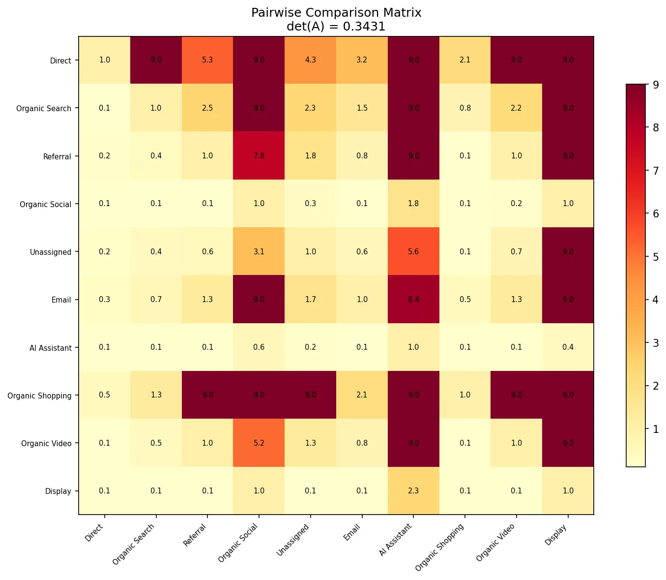
How to read it: read across a row. The cell at (Direct, Organic Search) is 9.0, so Direct dominates Organic Search across the metrics. Flip it around, and (Organic Search, Direct) is about 0.1, its reciprocal. Dark rows belong to channels that win a lot of matchups.
Step 2: Let the eigenvector settle it
Here’s the elegant part. Take the dominant eigenvector of this matrix, the one attached to the biggest eigenvalue, and normalize it to sum to 1. (np.linalg.eig does the work.) Each entry is that channel’s overall priority weight.
Why does that work? It’s the same idea as Google’s original PageRank. Beating a strong channel counts for more than beating a weak one, and the eigenvector is the one set of scores where every channel’s score agrees with the scores of the channels it beat. All 90 matchups get reconciled in one shot.
vals, vecs = np.linalg.eig(A)
top = np.argmax(vals.real)
weights = np.abs(vecs[:, top].real)
weights /= weights.sum()
Step 3: Sanity check (are the comparisons consistent?)
If A beats B and B beats C, then A should beat C. AHP checks for this with the consistency ratio. A perfectly consistent 10 × 10 matrix has a dominant eigenvalue of exactly 10, so the further above 10 you land, the more contradictions there are in your matchups.
- λ_max = 11.33
- Consistency ratio = 0.099 (the threshold is 0.10)
It passes, but only just. Keep that in mind.
The ranking
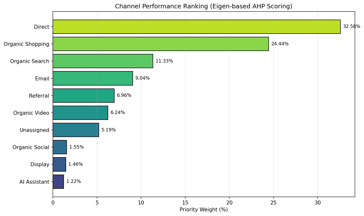
| Rank | Channel | Weight |
|---|---|---|
| 1 | Direct | 32.6% |
| 2 | Organic Shopping | 24.4% |
| 3 | Organic Search | 11.3% |
| 4 | 9.0% | |
| 5 | Referral | 7.0% |
| 6 | Organic Video | 6.2% |
| 7 | Unassigned | 5.2% |
| 8 | Organic Social | 1.6% |
| 9 | Display | 1.5% |
| 10 | AI Assistant | 1.2% |
Why you should care (and why you shouldn’t trust it blindly)
The interesting result is #2: Organic Shopping, with only 95 sessions. It wins on engagement rate, time on site and a healthy 6.3% key event rate, so in a head-to-head on quality it beats almost everyone. That’s a genuine signal: this is a channel worth testing more budget or feed optimization on. In a sessions-sorted report it’s buried at row 8.
Now be honest with yourself about what’s driving the rest:
- Direct is #1 partly because of Part 2. Sessions, Engaged sessions and Conversions are almost the same signal, and all three count equally here, so volume gets three votes. Re-run this with the redundant metrics dropped and Direct’s lead will shrink.
- Small channels swing hard. Organic Shopping’s 95 sessions and Display’s 13 produce ratio metrics that can jump around a lot from one week to the next. A 1-to-9 cap helps, but it doesn’t create sample size.
- “Higher is better” isn’t always true. The method treats longer engagement time as a win. Unassigned has the second-highest time on site (160s), but that’s almost certainly a tracking artifact, not delighted visitors.
- AI Assistant at the bottom is a “not yet,” not a “never.” 165 sessions and zero conversions is a small, new channel. Watch the trend; don’t kill it off a single snapshot. If you’re working on that channel, View as Markdown and Share with AI buttons are one cheap experiment.
The mental shortcut: use eigenvector ranking whenever you’re choosing among options on several criteria at once, like channels, vendors, campaign concepts or ABM target accounts. It beats a weighted average because it accounts for who you beat, not just your raw score. Always pair it with the redundancy check from Part 2 first, though. Garbage correlations in, biased rankings out.
Putting it together: a GA4 channel analysis workflow
Here’s the workflow, in the order you’d actually use it:
| Question | Tool | What it told us |
|---|---|---|
| Am I double-counting? | Correlation matrix + determinant | Yes. Engaged sessions = Sessions × Engagement rate, and conversions are mostly volume. |
| What are the real dimensions of performance? | PCA (eigenvalues/eigenvectors) | Three: volume, attention, conversion efficiency. |
| Which channels behave alike? | PCA biplot | Direct is unique; Shopping/Video/Referral form a “small but sticky” cluster. |
| What’s the overall ranking? | AHP eigenvector | Direct, then Organic Shopping (the hidden gem), then Organic Search. |
And here are the three habits worth stealing:
- Check for redundancy before you build anything. One
det()call can save you from a broken MMM or a biased scorecard. - Count dimensions, not KPIs. If three components explain about 90% of your data, your dashboard needs about three headline metrics. In this case: one for reach, one for attention, one for efficiency.
- Rank on matchups, not averages. When a channel wins on quality against strong competitors, the eigenvector notices, even if the sessions column doesn’t.
None of this needs a data science team. It’s a few dozen lines of NumPy on a CSV you already export every month. Download the full script, charts included (drawn with Matplotlib): analysis_slim.py, plus the sample data, traffic-data.csv. Put both files in one folder and run python analysis_slim.py. For more of this kind of analysis, see SEO keyword performance analysis with Python, Pandas and Matplotlib and finding low-hanging fruit in Google Search Console with regression and Bayesian models.
One last caveat, because you can handle it: this is 10 channels and one snapshot. That’s enough to show the method and get a few sharp hypotheses (look harder at Organic Shopping; stop reporting Engaged sessions next to Sessions; judge Email on rate, not count). It’s not enough to reallocate a budget on its own. Run it monthly, see which patterns hold, and then move money.