PyMC BAYESIAN ANALYSIS GUIDE FOR MARKETING DATA ANALYSTS

A Comprehensive Reference for Building Reliable Models.

Document version: 1.1
Last updated: December 2025
Target audience: Marketing analysts working with website traffic, signups, conversions, sales pipeline, channels, and campaigns.

CRITICAL SUCCESS FACTORS

These three rules are non-negotiable for every PyMC analysis:

1. ALWAYS check prior predictive distributions - Your model must make sense BEFORE seeing data.
2. ALWAYS choose distributions matching your data constraints - Count data needs count distributions, positive data needs positive distributions.
3. ALWAYS validate with posterior predictive checks - If your model cannot
   reproduce observed data, it is wrong.

THE COMPLETE BAYESIAN WORKFLOW

Follow these four stages in order. No shortcuts.

STAGE 1: Design Your Model

• Understand your data structure and constraints
• Choose appropriate likelihood distributions
• Specify priors based on domain knowledge

STAGE 2: Check Priors (Prior Predictive)

• Sample from priors before seeing data
• Verify simulated values are plausible
• If you see absurd extremes, tighten your priors

STAGE 3: Fit the Model (MCMC Sampling)

• Use sufficient draws, tuning steps, and chains
• Monitor convergence diagnostics
• Address any warnings immediately

STAGE 4: Validate Results (Posterior Predictive)

• Generate fake data from fitted model
• Compare to observed data
• If model cannot reproduce observations, it's wrong

DATA SANITY CHECK (Start Here Every Time)

Before building any model:

1. EXAMINE BASIC STATISTICS
   • Mean, variance, min, max
   • Standard deviation and range
   • Check for outliers
2. VERIFY DATA PROPERTIES
   • Units and any transformations
   • Presence of zeros or missing values
   • Data bounds and constraints
3. UNDERSTAND DATA TYPE
   • Is it counts (whole numbers only)?
   • Is it continuous and always positive?
   • Can it be negative?
   • Is it bounded (0-1, percentages)?
   • Is it binary (yes/no)?

CHOOSING THE RIGHT DISTRIBUTION

Match your distribution to your data constraints:

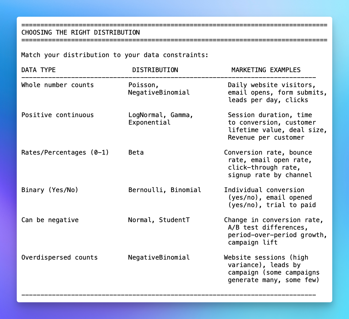
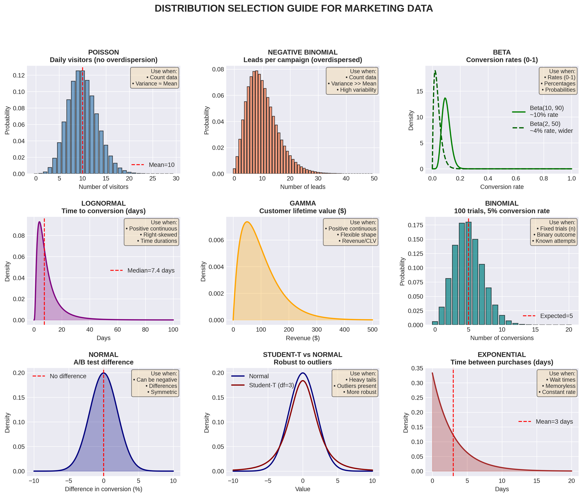
QUICK DECISION TREE:

1. Can I count it in whole numbers? → Poisson / NegativeBinomial
2. Is it always positive measurement? → LogNormal / Gamma
3. Is it a percentage or rate? → Beta
4. Is it just yes/no? → Bernoulli / Binomial
5. Can it be negative? → Normal / Student-T

MARKETING-SPECIFIC EXAMPLES:

Example 1: Daily Website Visitors

• Data: 450, 523, 389, 612, 501 visitors per day
• Type: Counts (whole numbers)
• Distribution: Poisson or NegativeBinomial
• Why NegativeBinomial? If variance >> mean (weekends vs weekdays vary a lot)

Example 2: Conversion Rate by Channel

• Data: Paid: 3.2%, Organic: 4.5%, Email: 5.1%
• Type: Percentage/rate (bounded 0-1)
• Distribution: Beta
• Prior example: Beta(2, 50) means ~4% with moderate uncertainty

Example 3: Time to First Purchase

• Data: 3.5 days, 12.1 days, 1.2 days, 45.3 days
• Type: Positive continuous (can't be negative)
• Distribution: LogNormal or Gamma
• Why LogNormal? Time data is often right-skewed

Example 4: Lead-to-Opportunity Conversion

• Data: 150 leads, 23 converted to opportunities
• Type: Binary outcomes
• Distribution: Binomial(n=150, p=?)
• Model learns: What's the conversion probability p?

Example 5: A/B Test Revenue Impact

• Data: Control mean $1,250, Treatment mean $1,310
• Type: Difference can be positive or negative
• Distribution: Normal for difference
• Goal: Is treatment > control?

COMMON PITFALLS TO AVOID

1. MIS-SPECIFYING PRIORS
   Bad: Using Normal(0, 1000) for a variance parameter
   Good: Using HalfNormal(5) for positive-only variance
   Remember: Priors must respect constraints (positive, bounded)
2. WRONG LIKELIHOOD FUNCTION
   Bad: Using Normal distribution for count data (e.g., daily signups)
   Good: Using Poisson or NegativeBinomial for counts
   Remember: Match distribution to data type.
   Marketing Example:
   Bad: Modeling email opens (counts) with Normal distribution
   Good: Modeling email opens with Poisson or NegativeBinomial
3. IGNORING CONVERGENCE DIAGNOSTICS
   Never ignore: Divergences, high R-hat, low ESS
   These mean: Your results are unreliable
   Action required: Fix before interpreting results
4. MISINTERPRETING RESULTS
   Don't: Treat credible intervals like confidence intervals
   Don't: Over-interpret point estimates
   Do: Report full uncertainty (credible intervals)
   Do: Acknowledge subjective prior choices. Key Difference:
   • Credible interval: "Given model + priors, there's X% probability
     parameter lies here."
   • Confidence interval: "In repeated sampling, X% of such intervals
     contain the true parameter."
5. INCOMPLETE POSTERIOR PREDICTIVE CHECKS
   Bad: Only checking mean predictions
   Good: Check entire distribution, tails, variance
   Remember: Model must reproduce all features of data.
   Marketing Example:
   Check if your model can generate both typical days (500 visitors) AND
   extreme days (2000 visitors from viral post)
6. FIXING VARIANCE WITHOUT JUSTIFICATION
   Bad: Setting sigma to a fixed value arbitrarily
   Good: Let the model learn variance from data
   Exception: Only fix if you have very strong domain knowledge.
   Marketing Example:
   Don't assume conversion rate variance is fixed at 0.01 unless you have
   strong historical evidence

SPECIFYING PRIORS CORRECTLY

GENERAL PRINCIPLES

1. RESPECT CONSTRAINTS
   • Use HalfNormal, HalfCauchy, Exponential for positive-only parameters
   • Use Beta for rates between 0 and 1
   • Never use unbounded priors for bounded parameters
   • Prefer HalfNormal / Exponential as defaults
   • Use HalfCauchy only when you intentionally want very heavy tails and
     you've checked prior predictive
2. USE DOMAIN KNOWLEDGE
   • Set realistic ranges based on subject matter expertise
   • Avoid overly tight priors unless strongly justified
   • Document your reasoning
     Marketing Examples:
• Website conversion rate: Beta(2, 50) suggests ~4% with uncertainty
• Daily visitors: NegativeBinomial with mu=500, alpha=10 if historical
  average is 500
• Email open rate: Beta(10, 90) suggests ~10% with moderate confidence
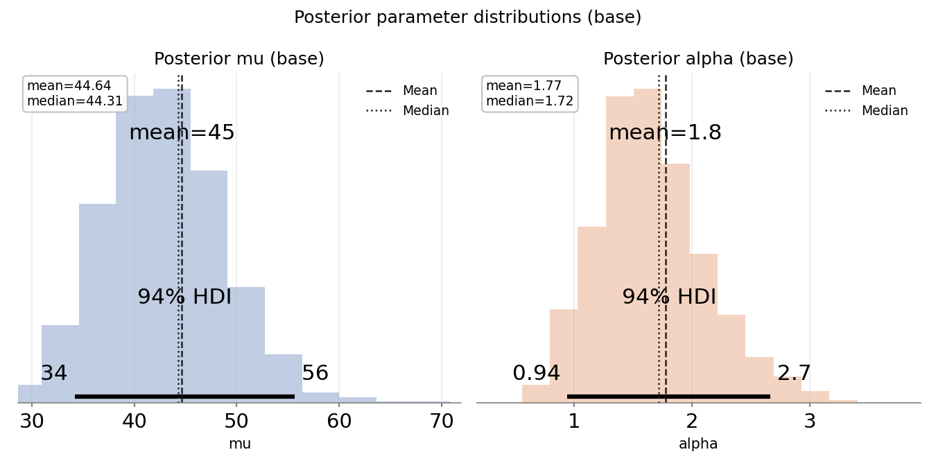
3. HANDLE CORRELATION AND WEAK IDENTIFICATION
   If parameters are highly correlated or weakly identified, consider
   reparameterization, stronger priors, or simplifying structure
4. CHECK PARAMETERIZATION
   Example: NegativeBinomial can be parameterized as (mu, alpha) or (n, p)
   • Understand what each parameter means (alpha, mu, sigma, etc.)
   • Verify formulas for mean, variance, overdispersion
   • Different distributions may use different parameterizations
• mu = mean, alpha = overdispersion
• Verify which parameterization your library uses!

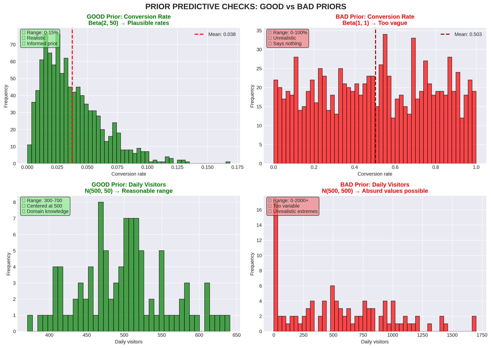
PRIOR PREDICTIVE WORKFLOW

1. Define priors
2. Sample from priors (before seeing data)
3. Generate simulated datasets
4. Ask: "Are these values plausible?"
5. If no → Adjust priors
6. Repeat until priors generate reasonable data

MARKETING PRIOR EXAMPLES

Email Campaign Open Rate:

• Prior: Beta(10, 90)
• Implies: ~10% open rate with some uncertainty
• Prior predictive: Generates rates between 5-20% (reasonable)

Daily Website Visitors:

• Prior: mu ~ Normal(500, 100), alpha ~ Exponential(0.1)
• Implies: Average around 500 visitors, moderate overdispersion
• Prior predictive: Should generate days between 200-1000 visitors

Conversion Rate by Channel:

• Prior for each channel: Beta(2, 50)
• Implies: Weak prior around 4%, allows learning
• Check: Does prior generate rates between 0.01-0.15? (reasonable for most
  channels)

Time to Conversion (days):

• Prior: LogNormal(mu=2, sigma=1)
• Implies: Median ~7 days (exp(2)), wide spread
• Prior predictive: Should generate times from 1 day to 100+ days

CONVERGENCE DIAGNOSTICS (Must-Check List)

1. R-HAT (GELMAN-RUBIN STATISTIC)
   Target: ≤ 1.01 (ideally 1.00-1.01)
   Meaning: Do all chains agree on the same distribution?
   If > 1.01: Chains disagree; run longer or reparameterize
   Action: Increase draws/tune or fix model structure
2. EFFECTIVE SAMPLE SIZE (ESS)
   Target: Hundreds+ for stable estimates
   Meaning: How many independent samples do we have?
   If < 100: Chain is sluggish, autocorrelation is high
   Action: Increase draws or improve parameterization
3. DIVERGENCES
   Target: 0 (zero divergences)
   Meaning: Sampler hit trouble spots in posterior
   If > 0: Sampler is missing important posterior regions
   Action:
   • Increase target_accept (try 0.95 or 0.99)
   • Reparameterize model (non-centered parameterization)
   • Simplify model structure

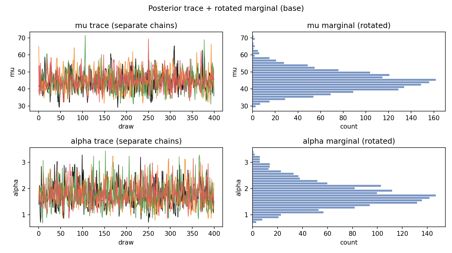
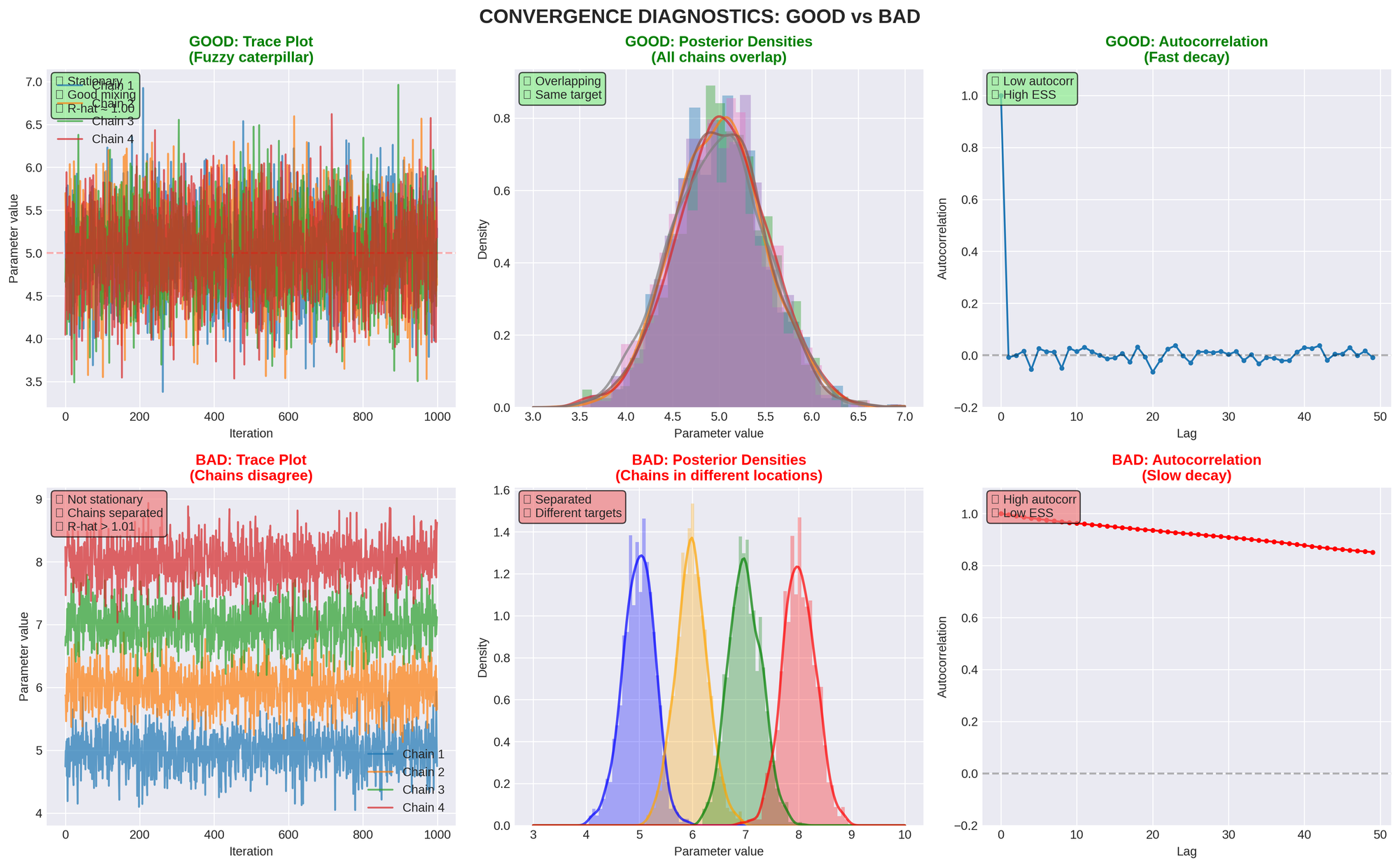
VISUAL DIAGNOSTICS

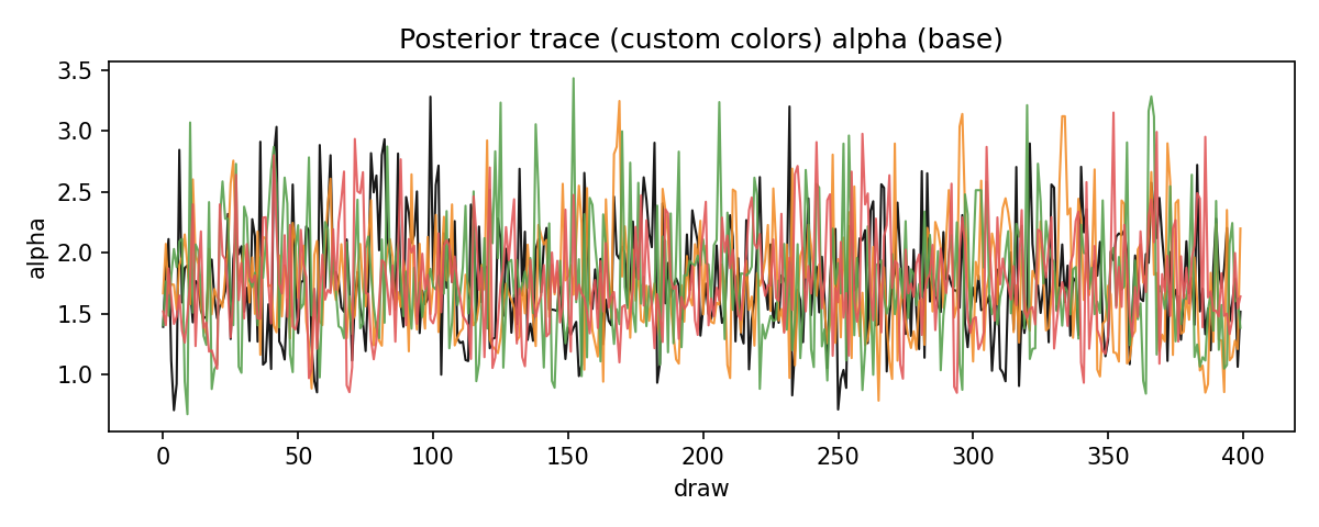
TRACE PLOTS

• Good: Chains look like "fuzzy caterpillars"
• Bad: Chains show trends, drift, or distinct bands
• Look for: Stationarity, mixing, convergence

RANK PLOTS

• Good: Uniform distribution across ranks
• Bad: Patterns or clustering in ranks
• Better than: Traditional trace plots for detecting issues

CHAIN COMPARISON (KDE PLOTS)

• Good: All chains have overlapping distributions
• Bad: Chains sit in different locations
• Indicates: Convergence problems if separated

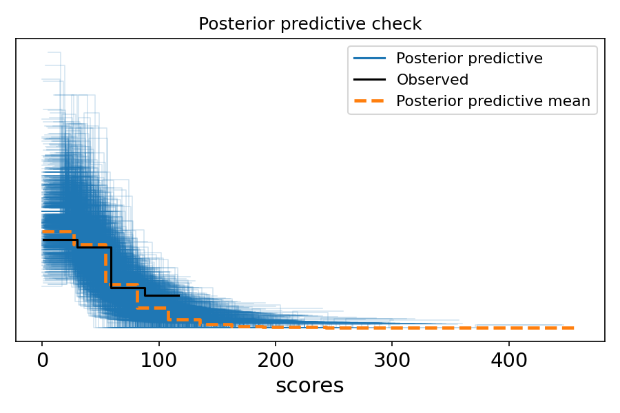
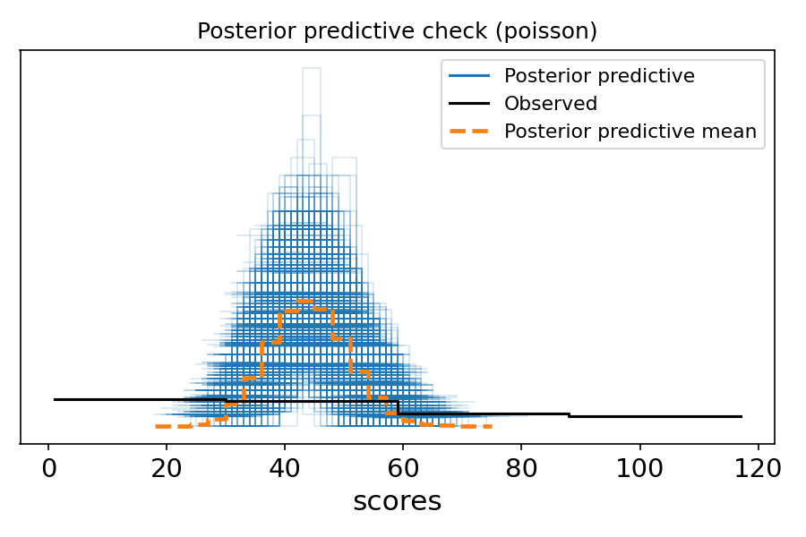
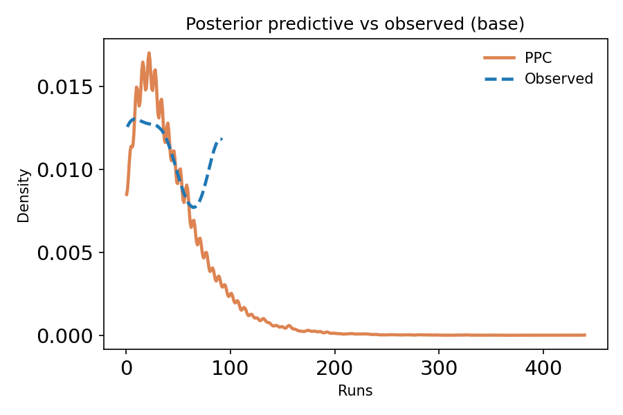
POSTERIOR PREDICTIVE CHECKS (PPC)

PURPOSE

Verify that your fitted model can reproduce the observed data.

WHAT TO CHECK

1. Central tendency: Does model match observed mean/median?
2. Spread: Does model capture observed variance?
3. Tails: Can model generate extreme values seen in data?
4. Shape: Does overall distribution match?
5. Coverage: Are observed totals within predicted range?

INTERPRETATION

• Good PPC: Observed data looks typical compared to predictions
• Bad PPC: Observed data is extreme or outside predicted range
• Action if bad: Model is wrong; revise and refit

COMMON PPC FAILURES

• Under-fit tails: Use heavier-tailed distribution (e.g., StudentT instead
  of Normal)
• Under-dispersed: Use NegativeBinomial instead of Poisson
• Wrong central tendency: Check likelihood specification
• Systematic bias: Missing predictors or wrong functional form
• Overlay histogram/density of observed vs simulated
• Time series overlay (if data is temporal)
• Also: Check coverage: what % of observed points fall inside 50% / 90%
  predictive intervals?

MARKETING PPC EXAMPLES

Example 1: Daily Visitor Model

• Check: Can model generate both typical days (400-600) AND peak days
  (1500+)?
• Check: Does model capture day-of-week effects if present?
• Check: Are 90% of observed days within model's 90% predictive interval?

Example 2: Conversion Rate Model

• Check: Does model predict rates consistent with historical performance?
• Check: Can model capture variation between channels?
• Check: Does model handle campaigns with very few conversions?

Example 3: Email Campaign Performance

• Check: Does model reproduce observed open rates across campaigns?
• Check: Can model handle campaigns with high engagement (15%+) and low
  engagement (2%)?
• Check: Does model account for list fatigue over time?

PERFORMANCE OPTIMIZATION

PREFER NUMPYRO NUTS WHEN AVAILABLE

Setup:

from pymc.sampling.jax import sample_numpyro_nuts
import os

Set cache directories to avoid permission issues

os.environ['MPLCONFIGDIR'] = '.matplotlib_cache'
os.environ['PYTENSOR_FLAGS'] = 'compiledir=.pytensor_cache'

Sampling Parameters:

• draws: ≥ 400 (1000+ recommended)
• tune: ≥ 400 (1000+ recommended)
• chains: ≥ 4
• target_accept: 0.9 (0.95 for difficult geometries)
• chain_method: "parallel"

ADVANTAGES OF NUMPYRO NUTS

1. No C++ compilation issues (uses JAX backend)
2. More efficient than Metropolis-Hastings
3. Better automatic adaptation and tuning
4. Proper convergence with multiple chains
5. GPU acceleration available
6. Faster execution overall

FALLBACK STRATEGY

• First choice: NumPyro NUTS with full data
• If unavailable: PyMC NUTS with reduced draws/tune
• Ensure: PyMC version exposes pymc.sampling.jax
• Warning: PyMC NUTS is slower than NumPyro

SAMPLING BEST PRACTICES

• Use full dataset (don't subset for speed)
• Run minimum 400 draws + 400 tune with 4 chains
• Watch diagnostics: R-hat ≤ 1.01, ESS high, divergences = 0
• Rerun with more draws/chains if thresholds not met
• Select draws/tune/chains to ensure valid fit

MODEL COMPARISON

LEAVE-ONE-OUT CROSS-VALIDATION (LOO)

What to check:

1. ELPD_LOO (EXPECTED LOG POINTWISE PREDICTIVE DENSITY)
   • Higher (less negative) is better
   • Difference > 10 is meaningful
   • Measures out-of-sample predictive accuracy
2. P_LOO (EFFECTIVE NUMBER OF PARAMETERS)
   • Should be close to actual parameter count
   • Very large values indicate overfitting or missing noise term
   • Unusually high = model forcing structure on data
3. PARETO-K DIAGNOSTIC
   • Must be < 0.7 for reliable results
   • k > 0.7 means LOO estimates are unreliable
   • Action if k > 0.7: Fix model before trusting results

RULES OF THUMB

• Large elpd_loo difference (>10) = meaningful improvement
  Consider Δelpd relative to its SE (if Δelpd is small vs SE, don't
  overclaim)
• p_loo unusually high = model complexity warning
  p_loo is an effective complexity measure; unusually high values can
  indicate overfitting, weak priors, or a missing noise term
• Any Pareto-k > 0.7 = results unreliable

MARKETING EXAMPLE: COMPARING CAMPAIGN MODELS

Model A: Simple Poisson for daily leads

• elpd_loo = -850.2
• p_loo = 2.1 (close to 2 parameters)
• Pareto-k: all < 0.5 (good)

Model B: NegativeBinomial with channel effects

• elpd_loo = -825.7
• p_loo = 5.3 (close to 5 parameters)
• Pareto-k: all < 0.6 (good)

Conclusion: Model B is better (elpd_loo difference = 24.5 >> 10)
The extra complexity is justified by improved predictions

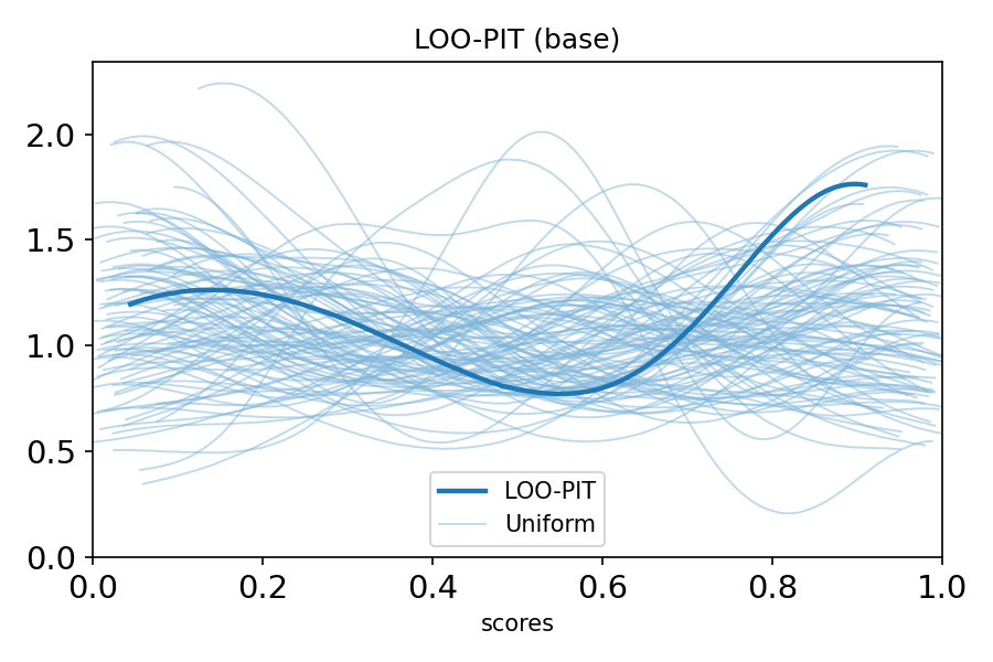
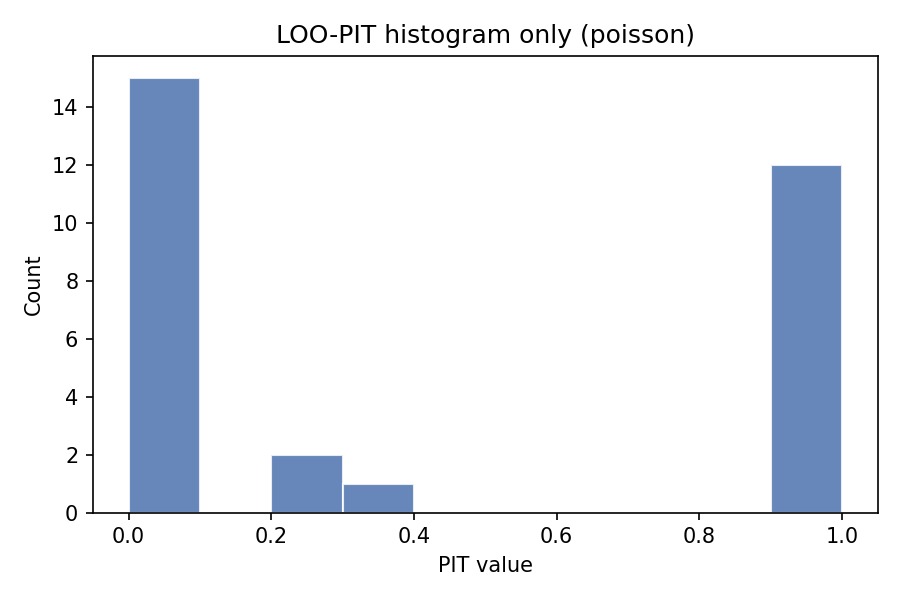
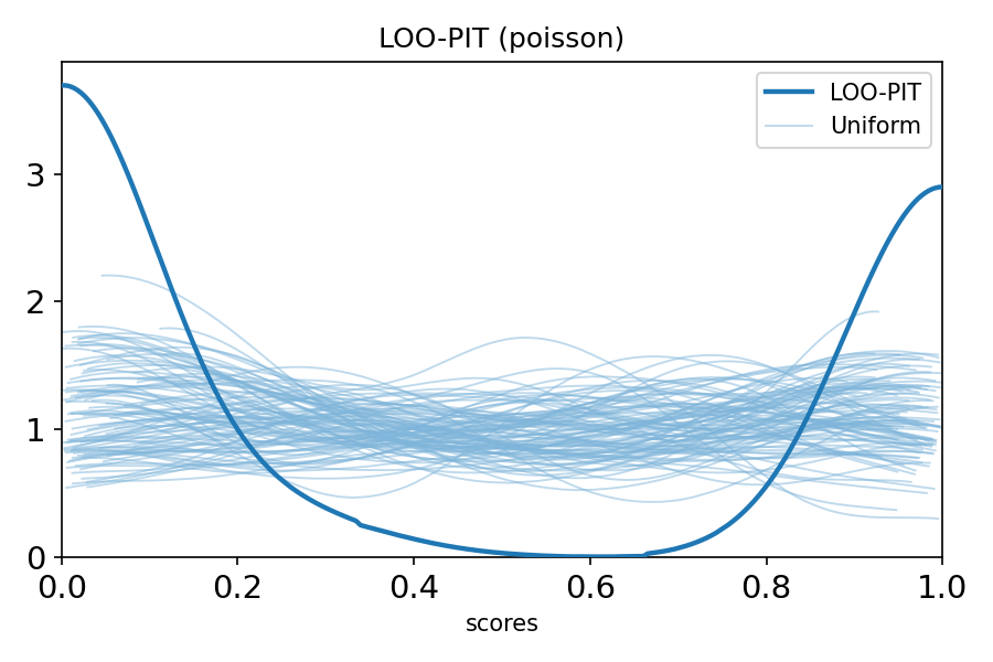
LOO-PIT (PROBABILITY INTEGRAL TRANSFORM)

Purpose: Check whether your model has realistic uncertainty

What it checks:

• Does model predict unseen data well?
• Is model over-confident or under-confident?
• Are predictions properly calibrated?

Interpretation:

• Uniform distribution = well-calibrated
• U-shaped = over-confident (intervals too narrow)
• Inverse-U = under-confident (intervals too wide)

WAIC (WIDELY APPLICABLE INFORMATION CRITERION)

When to use:

• Alternative to LOO when log-likelihood is available
• Compute: az.waic(idata)
• Compare elpd_waic: higher (less negative) is better

Warnings:

• If var(log p) > 0.4, WAIC may be unreliable
• Prefer LOO if WAIC shows warnings

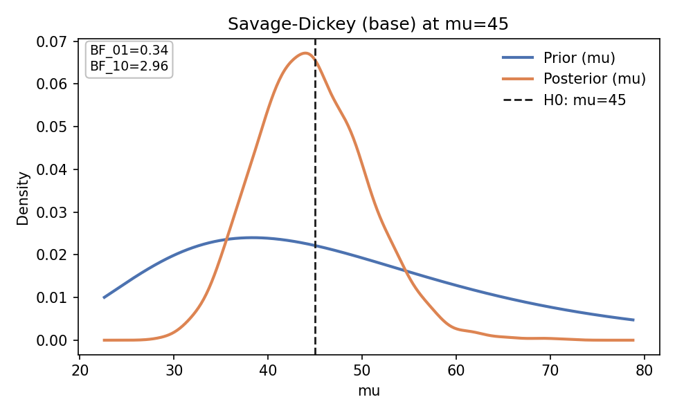
SAVAGE-DICKEY BAYES FACTOR

Use case: Testing point-null hypothesis in nested models

Requirements:

• Proper priors (not improper)
• Nested model structure
• Testing specific parameter value

Computation:
BF_01 = prior_density(theta=0) / posterior_density(theta=0)

Interpretation:

• BF ~ 1: Weak evidence
• BF 3-10: Moderate evidence
• BF > 10: Strong evidence
• BF < 1/3: Evidence against null

Marketing Example:
Testing if paid search has zero effect on conversions

• If BF_01 > 10: Strong evidence of no effect
• If BF_01 < 1/3: Strong evidence of positive effect

COMPLETE DIAGNOSTIC CHECKLIST

Use this checklist for every model:

BEFORE FITTING

[ ] Data sanity check completed
[ ] Distribution matches data constraints
[ ] Priors specified with justification
[ ] Prior predictive check shows reasonable values
[ ] Parameterization verified (mu, alpha, sigma meanings)

DURING FITTING

[ ] Used NumPyro NUTS if available
[ ] Set appropriate draws/tune/chains
[ ] Cache directories configured
[ ] Sampling completed without errors

AFTER FITTING (CONVERGENCE)

[ ] R-hat ≤ 1.01 for all parameters
[ ] ESS > 100 (preferably hundreds+) for all parameters
[ ] Divergences = 0
[ ] Trace plots show good mixing
[ ] Rank plots show uniform distribution
[ ] Chains converge to same distribution

VALIDATION

[ ] Posterior predictive check performed
[ ] PPC shows model reproduces observed data
[ ] PPC covers central tendency, spread, and tails
[ ] LOO computed and Pareto-k < 0.7
[ ] LOO-PIT shows proper calibration
[ ] WAIC computed if appropriate

MODEL COMPARISON (IF APPLICABLE)

[ ] Compared to simpler baseline model
[ ] elpd_loo differences computed
[ ] p_loo values reasonable
[ ] Best model selected with justification

REPORTING

[ ] Report full credible intervals (not just point estimates)
[ ] Acknowledge uncertainty
[ ] Document prior choices
[ ] Note any model limitations
[ ] Avoid over-interpreting results

WARNING SIGNS & FIXES

BAD CHAINS (SYMPTOMS)

• Chains sit in different bands
• Chains drift over time
• Distinct KDEs for different chains
• High R-hat values

Why this happens:

• Multimodal posterior
• Poor geometry (funnel, high correlation)
• Misspecified priors/likelihood
• Weak identifiability
• Insufficient tuning/draws
• Too-low target_accept

Fixes:

1. Increase draws and tuning steps
2. Increase target_accept to 0.95 or 0.99
3. Reparameterize (try non-centered parameterization)
4. Simplify model structure
5. Check prior specification

IMPORTANT REMINDER: GOOD CHAINS ≠ GOOD MODEL

Even with R-hat ~ 1.00 and zero divergences, your model can still be wrong if:

• PPC fails (model can't reproduce data)
• Wrong likelihood chosen
• Missing important predictors
• Incorrect functional form

Always validate with posterior predictive checks!

• If prior predictive is implausible → stop
• If posterior predictive misses key features (variance, tails,
  seasonality) → stop

THE BIG PICTURE (ELI5)

Think of PyMC like this:

1. WRITE YOUR GUESS (story about the world)
   What kind of data-generating process makes sense?Marketing Example: "I think conversion rate is around 3-5% with some
   variation by channel"
2. CHECK IF IT'S SILLY (before looking at data)
   Would your guess make reasonable fake data?Example: Does your prior generate conversion rates between 0-20%?
   (Reasonable) or between -10% to 150%? (Silly!)
3. UPDATE YOUR GUESS (using real data)
   Let the data teach you what actually fitsExample: Data shows organic channel converts at 7%, paid at 2.5%
4. TEST IF IT WORKS (generate fake data and compare)
   Can your updated guess make data like the real thing?Example: Can your model generate both high-converting days and
   low-converting days?

THE MAGIC

• Starts with your guess (priors)
• Looks at real data (likelihood)
• Updates to what actually fits (posterior)
• Maybe it learns something new!

GOLDEN RULES

1. Follow the 4-stage workflow
   Design → Check Priors → Fit → Validate. No shortcuts.
2. Match distributions to data constraints
   Count data needs count distributions, not Normal.
3. Let the model learn variance
   Never fix sigma unless you have very strong domain knowledge.
4. Always validate
   If posterior predictions don't match observed data, your model is wrong.
5. Never ignore convergence warnings
   Divergences and high R-hat mean invalid inference.
6. Check parameterization
   Always verify parameter meanings before sampling.
7. Use domain knowledge
   Set realistic priors based on subject matter expertise.
8. Report uncertainty
   Always include credible intervals, never just point estimates.
9. Compare alternatives
   Try simpler baseline model first (e.g., Poisson before
   NegativeBinomial).
10. Interpret with humility
    Don't over-interpret single point estimates. Acknowledge limitations.

MARKETING-SPECIFIC MODELING SCENARIOS

SCENARIO 1: WEBSITE TRAFFIC MODELING

Business Question: What's our expected daily traffic next month?

Data Characteristics:

• Whole number counts (visitors per day)
• Likely overdispersed (weekends differ from weekdays)
• Possible seasonality

Recommended Approach:

1. Distribution: NegativeBinomial (handles overdispersion)
2. Priors:
   • mu ~ Normal(current_avg, current_std)
   • alpha ~ Exponential(0.1) for overdispersion
3. Add day-of-week effects if needed
4. Validate: Can model reproduce both slow days and peak days?

Red Flags:

• Poisson under-fits if weekday/weekend variance is high
• Check PPC for tail coverage

SCENARIO 2: A/B TEST FOR CONVERSION RATE

Business Question: Is new landing page better than control?

Data Characteristics:

• Binary outcomes (converted: yes/no)
• Two groups to compare
• Need probabilistic statement about difference

Recommended Approach:

1. Distribution: Binomial(n, p) for each variant
2. Priors: Beta(2, 50) for both p_control and p_treatment (weak prior ~4%)
3. Compare posteriors: P(p_treatment > p_control)
4. Report: Full credible interval for difference

Red Flags:

• Don't just report "treatment won" - report probability and magnitude
• Check if difference is practically significant (not just statistically)

SCENARIO 3: CUSTOMER LIFETIME VALUE (CLV)

Business Question: What's the expected revenue per customer?

Data Characteristics:

• Positive continuous (revenue can't be negative)
• Often right-skewed (most customers spend little, few spend a lot)
• May have high variance

Recommended Approach:

1. Distribution: LogNormal or Gamma
2. Priors:
   • LogNormal: mu ~ Normal(log(historical_avg), 0.5)
   • sigma ~ HalfNormal(1)
3. Consider segment-specific models (new vs returning)
4. Validate: Can model generate both typical and high-value customers?

Red Flags:

• Normal distribution will predict negative CLV (impossible!)
• Check if tails are well-modeled in PPC

SCENARIO 4: CAMPAIGN PERFORMANCE ACROSS CHANNELS

Business Question: Which channels perform best for lead generation?

Data Characteristics:

• Count data (leads per campaign)
• Multiple groups (channels)
• Likely different variances per channel

Recommended Approach:

1. Distribution: NegativeBinomial (channel-specific)
2. Hierarchical structure:
   • Overall mean across channels
   • Channel-specific deviations
3. Priors: Weakly informative based on historical channel performance
4. Validate: Model should capture both high-performing and low-performing
   campaigns

Red Flags:

• Don't assume all channels have same variance
• Check if model handles channels with very few campaigns

SCENARIO 5: EMAIL CAMPAIGN OPEN RATES

Business Question: What's our true open rate, accounting for uncertainty?

Data Characteristics:

• Rate/percentage (bounded 0-1)
• Multiple campaigns to aggregate
• Want credible interval, not just point estimate

Recommended Approach:

1. Distribution: Beta-Binomial (for each campaign)
2. Hierarchical model:
   • Overall open rate (Beta prior)
   • Campaign-specific variation
3. Priors: Beta(10, 90) suggests ~10% with moderate confidence
4. Validate: Does model handle both high-engagement and low-engagement
   campaigns?

Red Flags:

• Point estimate hides uncertainty - always report full posterior
• Check if list fatigue (declining open rates over time) needs modeling

SCENARIO 6: TIME TO CONVERSION

Business Question: How long until leads convert to customers?

Data Characteristics:

• Positive continuous (days/hours)
• Right-skewed (most convert quickly, some take long)
• May have censoring (leads that haven't converted yet)

Recommended Approach:

1. Distribution: LogNormal or Weibull
2. Consider survival analysis if censoring is important
3. Priors:
   • LogNormal: mu ~ Normal(log(7), 1) if median is ~7 days
   • sigma ~ HalfNormal(1)
4. Validate: Can model generate both quick conversions (1 day) and slow
   conversions (60+ days)?

Red Flags:

• Exponential assumes constant hazard (may be unrealistic)
• Check if there are distinct "fast" and "slow" converter populations

PRACTICAL TIPS FOR MARKETING ANALYSTS

1. START SIMPLE, ADD COMPLEXITY AS NEEDED
   • Begin with basic model (e.g., Poisson for counts)
   • Add overdispersion if needed (NegativeBinomial)
   • Add predictors only if they improve LOO significantly
2. USE HISTORICAL DATA TO INFORM PRIORS
   • If average conversion rate is 3-5% historically, use Beta(3, 97) prior
   • If daily traffic averages 500, center prior around mu=500
   • Don't use uninformative priors when you have domain knowledge
3. THINK IN TERMS OF DATA-GENERATING PROCESSES
   • How does the world generate this data?
   • What constraints must be respected?
   • What sources of variation exist?
4. VALIDATE AGAINST BUSINESS INTUITION
   • Does predicted conversion rate match your experience?
   • Are forecasts reasonable given market conditions?
   • Can stakeholders understand and trust your uncertainty estimates?
5. COMMUNICATE UNCERTAINTY CLEARLY
   • Report: "Conversion rate is 3.2% [95% CI: 2.8-3.6%]"
   • Not: "Conversion rate is 3.2%"
   • Show stakeholders the full posterior distribution when possible
6. COMPARE TO FREQUENTIST BENCHMARKS
   • Run traditional t-tests or proportion tests as sanity checks
   • Bayesian results should be in same ballpark (if using weak priors)
   • If very different, understand why
7. DOCUMENT YOUR MODELING CHOICES
   • Why this distribution?
   • Why these priors?
   • What assumptions are made?
   • What are the limitations?
8. ITERATE AND IMPROVE
   • First model is rarely final model
   • Use PPC to identify weaknesses
   • Add complexity only when justified by data

FINAL WORDS:

Bayesian analysis is powerful but requires discipline. Every shortcut risks
invalid inference. Follow this guide systematically, and you'll build
reliable models that produce trustworthy results.

WHEN IN DOUBT:

• Check your data first
• Pick the right "number-making machine"
• Make a reasonable starting guess
• Test the machine before and after training
• If the machine can't copy real data, fix it
• Always verify parameter meanings

REMEMBER: A model that passes all diagnostics can still be wrong if it fails
posterior predictive checks. Validation is not optional.

Good luck with your analyses!

BAYESIAN QUICK REFERENCE CARD

WORKFLOW CHECKLIST:
[ ] 1. Sanity check data
[ ] 2. Choose distribution matching data type
[ ] 3. Set informative priors from domain knowledge
[ ] 4. Prior predictive check (before fitting)
[ ] 5. Fit with NumPyro NUTS (draws≥400, chains≥4)
[ ] 6. Check R-hat≤1.01, ESS>100, divergences=0
[ ] 7. Posterior predictive check (after fitting)
[ ] 8. Compare models with LOO if needed
[ ] 9. Report full uncertainty (credible intervals)
[ ] 10. Document all choices and limitations

CONVERGENCE TARGETS:

• R-hat: ≤ 1.01
• ESS: Hundreds+ (minimum 100)
• Divergences: 0
• Pareto-k: < 0.7

DISTRIBUTION QUICK REFERENCE:

• Daily visitors (counts): NegativeBinomial
• Conversion rate (0-1): Beta
• Time to convert (positive): LogNormal
• Yes/no conversion: Binomial
• Revenue difference: Normal
• Overdispersed counts: NegativeBinomial

WHEN MODEL FAILS:

1. Check prior predictive (silly priors?)
2. Check convergence (bad chains?)
3. Check posterior predictive (wrong likelihood?)
4. Simplify or reparameterize
5. Try different distribution family

REPORTING TEMPLATE:
"We estimate [parameter] is [point estimate] with 95% credible interval
[lower, upper]. This means there's a 95% probability the true value lies
in this range, given our model and data. Key assumptions: [list].
Limitations: [list]."